There are many different tools available for tracking projects, each of which can help with planning and scheduling work. Sometimes, though, there is room for a simple high-level plan. Excel can be a great tool to use to create this.
There are so many different project management tools that can create plans of different types, or help to assign and track work etc. Sometimes though I find it useful to create a basic plan to act as a visual aid for scheduling and risk management. This can be particularly useful if you want to maintain visibility of activity or events external to your team. For example, I worked on a large web project where we would add in high level marketing communication activity to make sure we weren’t planning to revamp the login/registration pages at the same time as a major media campaign driving traffic to the site.
Excel can be a great tool for producing this sort of plan. I am going to walk through the creation of a template that I use when drawing up these plans. The template contains a few different tricks and techniques for working with dates in Excel. Hopefully it might give you a bit of inspiration in the things you can get Excel to do.
We will build the template using the following;-
- Built in Date Picker component to set start date of the plan
- Basic Excel functions to populate our horizontal date axis
- Conditional Formatting to highlight weekends months etc
- A custom function to add month names to our horizontal date axis
- A nice vertical line marker to highlight a date
- Some macros to move this line about as required
Basic Spreadsheet and Datepicker set up
Open up a spreadsheet and make sure the Developer tab is visible. If it is not go to File > Options > Customize Ribbon and make sure Developers tab is checked in the right hand panel.

Go to the Developers tab and click on Insert. From the resulting drop-down panel, select the bottom right ‘More Controls’ option.
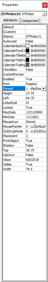
Select the Microsoft Date and Time Picker control, and then add it to the top left of your spreadsheet – I have it around cell B3.

Make sure that Design Mode is switched on on the Developers tab. If you right click on the date picker object you can select the properties for this control.
About two thirds of the way down the list of properties you should the ‘LinkedCell’ property. Enter I5 to link the control to a cell on your spreadsheet and then give yourself a pat on the back!
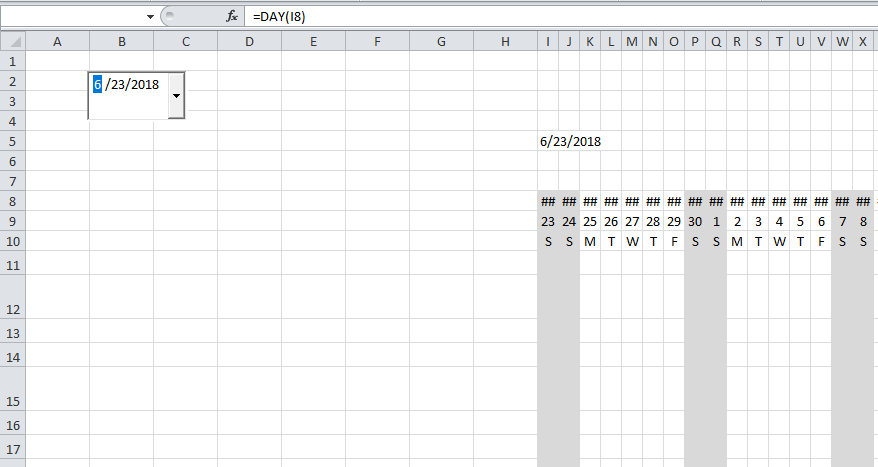
Now you can select dates in the date picker and see the selected date appear on the spreadsheet! But this is text string, which is not so useful for us. We can use the VALUE function to convert this to a number. In cell I8 type
=VALUE(I5)
and we get the text output of the Date Picker converted to an Excel Date number.
in cell J8 type
=I8+1
to increment this date. You can then copy J8 out to the right a bit to put incremental date number in row 8. This will form the basis of our plan.

Tidy up the spreadsheet and prepare for more formualae
The next step is to resize some rows and columns. We want to shrink down our columns a bit to make our plan more visible and manageable. Select columns I to GZ and make them all 2.29 (21px) wide. That will extend our plan out to 200 days, which should be sufficient.
Rows from row 11 down will contain details of the activity and events appearing on our plan. I set up the rows in groups of three – the second of three to contain task bars and milestones etc, and the first and third to act as spacing rows. I do this because it gives me flexibility in formatting but you can set this part of the plan up in whichever way suits you.
So I resize rows 11 and 13 to 18.00 (24px) and row 12 to 33.00 (44px). I can then copy there three rows and paste them down further to make expand the rows in my plan.
If we add a shape to our plan (Insert > Shapes) we can access the Drawing Tools > Format tab. Under Align tools there is an option to Snap to Grid. We can now make our shapes snap neatly to the gird of cells we have just created.
Enhance our timeline with simple formula
Lets spruce our timeline up with a couple of simple formulae.
firstly copy the formula in cell J8 out to populate out 200 days worth of columns. Copy J8 (=I8+1) to cells (K8:GZ8). This row of Date Numbers is going to drive our entire timeline.
Then in cell I9 enter
=DAY(I8)
This will take our date number and return the day of the month. Copy this formula to cells J9:GZ9 and you should see the days of the month for all our columns. Pretty nifty stuff! You can experiment changing the date using the date picker control and see the days of the month change accordingly.
We definitely want to be able to see which days of the week correspond to these days of the month. We are going to use a VLOOKUP function for this step.
The VLOOKUP is one of the most useful Excel functions but it requires a bit of set-up.
Click on another tab to go to another worksheet within the same document. We are going to create a little table of data and use a vlookup function to pull information through to our timeline.
You need to create a little table of data, two columns wide and eight rows deep. The top row holds titles, the rest of the first column the numbers 1-7, the rest of the second column, “M”,”T”,”W”,”T”,”F”,”S”,”S”.
Select this little table and give it a name, something like “weekday_text” in the field just above the top left corner of your worksheet.

Skip back to your main plan worksheet and go to cell I10. We are going to write a formula that looks at the date number for this column (in cell I8). We are going to use the WEEKDAY function to return a number from 1 to 7 that corresponds with the day of the week. We will then use a VLOOKUP function to take this number and return a single letter from our weekday_text table.
type in “=WEEKDAY(I8,2)”. Copy this forumla along the row and you will see numbers repeating from 1-7, corresponding with days of the week.
We need to nest this in a VLOOKUP to convert it to a letter from our table. Go to cell I10 and add in “VLOOKUP(” following between the “=” and the WEEKDAY function. This starts our function, and specifies the first parameter, the number that we want to look up.
We can complete the final three parameters, the table we want to lookup in, the return column number, and whether we want an exact match. At the end of your weekday function add the following, “,weekday_text,2,FALSE)” and hit return. This should now be taking our weekday number, looking it up in our table and returning the correct letter from column 2.

Add a bit of conditional formatting
What we really need now is some visual cue to highlight weekend days
We can use Conditional Formatting to achieve this – we can change the fill color of weekend cells, and makes this change dynamically if we change the start date of our timeline.
Click on any cell in the main part of the plan, for example I9. Now click on the Conditional Formatting command on the Home Tab and select New Rule to display the conditional Formatting window.
Select “Use a Formula to determine which cells to format”.
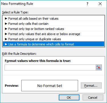
Excel will apply some special formatting to the cell when our formula evaluates as true. We want a formula that evaluates as true for ‘weekend’ cells. We can use our weekday function on cell I8 to return our number from 1-7 and evaluate as true for numbers 6 & 7. We write this as “=WEEKDAY(I8,2)>5”.
So far so good, but we want to apply this formula to our entire range. For any cell we want the formula to return a weekday number based on row 8 of current column and evaluate a TRUE if it is over 5. We just need to add in a “$”before the 8 to make sure this becomes an absolute reference. So we get “=WEEKDAY(I$8,2)>5”.
Once you OK the formula you can specify a format for these cells – click on the Format rectangle and add a light grey fill to these cells.
You can then specify the cells it should apply to. I have it applying to “=$I$9:$GZ$115”. If you then click on OK you should see your light grey formatting applied to all the Saturday and Sunday columns on your plan. And if you change the Start Date with your Date Picker control it should all update automatically!